sicr
Stochastic Individual Claims Reserving
Dirk Skowasch
2025-11-15
sicr.RmdAbstract
The sicr package provides functions to apply the stochastic individual claims reserving method to a group of claims for the purpose of estimating future payments.Introduction
Motivation
This package implements the stochastic individual claims reserving (sicr) that was first published by Dirk Skowasch and Torsten Grabarz (see 08.03.2022 on https://www.qx-club.de/ARCHIV/). It is based on the paper of Murphy & McLennan but extends it in some areas for better applicability under Solvency II.
The basic idea is that the year-to-year development of every single large claim is sampled from a pool of historic observations of similar claims. Repeating this will lead to a monte carlo simulation from which best estimates for future gross and reinsurance payments can be derived.
The most significant extensions and differences to Murphy/McLennan are
- the use of reserve classes to classify open claims.
- the focus on absolute payments instead of development factors, thus indexation is required.
- the consideration of annuities.
This vignette offers a step by step guide to use the package. It also includes some technical explanations, but does not offer a detailed description of the method. This can instead be found in the above linked article.
General information in advance
Payment and reserve matrices
At some points development triangles are used and filled up to rectangles.
This package (with very few exceptions) always uses the calendar year representation, which means that rows represent origin years and columns represent calendar years.
Payment entries are always incremental. Reserve entries resemble the reserve at the end of the column’s calendar year.
A triangle might look like this:
all_claims_paid_xmpl[29:35,29:35]## 2017 2018 2019 2020 2021 2022 2023
## 2017 15288846 7429705 2123140 1675310 969867.8 883693.2 582269.2
## 2018 0 14780727 9539884 3850741 1949593.0 1541325.2 641839.2
## 2019 0 0 12786517 7235091 2565975.7 1547881.4 1107299.4
## 2020 0 0 0 12136297 5887067.4 1881856.9 1826378.6
## 2021 0 0 0 0 9233157.4 6245616.2 3151468.0
## 2022 0 0 0 0 0.0 10496593.6 6040388.9
## 2023 0 0 0 0 0.0 0.0 9834412.8Dividing into small, large and special claims
A claim is considered large if its cumulated indexed
payments plus its latest indexed reserve exceed the chosen
threshold.
Note that only payments after and in the year that the claim
exceeded the threshold will be considered as large claim payments. All
payments before belong to small claims.
Large claims payments are projected with the stochastic individual
claims reserving method.
Some claims might be extraordinarily large (or different in any other way) so that there haven’t been enough similar historic observations that can be used to project them with. These claims are called special claims. They are seperated from the rest and projected deterministically (see description below).
We obtain small claims payments and reserves triangles by subtracting large and special claims’ development triangles from the overall development triangles.
Annuities
In some countries it is common to convert recurring payments into
annuities. Usually the actuary then gets access to some additional
biometric information about the annuity recipient that can be used to
improve the estimate of future payments. This package allows for the
separate treatment of annuities, but some extra input dataframes and
matrices will be required. In that case, dataframe columns like
Cl_payment_cal (for claims payments in one specified
calendar year) do not include annuity payments as they are included in
An_payment_cal. If annuities are irrelevant or are
considered as common claim payments, all annuity columns must be 0 and
the annuity dataframes can be set to NULL.
IBNR claims
IBNR claims are calculated as described in the paper with an additive method for the number and a sampling from historic IBNR large claims for the amount of each expected claim. Two parameters need to be selected as input for the IBNR method:
- The dataframe
exposurewill be used for the additive method and is described below. - The vector
years_for_ibnr_poolscontains the calendar years that shall be used to build the pools to sample the amount from.
Both parameters will be needed in the function sicr().
They may also be NULL, in that case a constant exposure and all observed
calendar years will be used.
Reinsurance
The method can be applied on a gross basis without reinsurance by
setting the reinsurance dataframe to NULL, but this would
deprive the method of one of its main advantages. If reinsurance shall
be included, the help of the function xl_cashflow()
provides detailed information about how the dataframe
reinsurance needs to be structured. Furthermore, the
dataframe historic_indices resp. indices must
contain the column Index_re, see help of
indices_xmpl.
Matrix naming convention
With the above stated, it is useful to introduce a naming convention:
A payments or reserve matrix’ name consists of three parts, each
separated by an underline, e.g. large_claims_paid.
- The first part is one of
allsmall-
largeor -
special
and describes where the claim belongs to.
- The second part is either
-
claimsor -
annuities
depending on whether the payment (or reserve) is a pure claims payment (that means without annuity payments) or an annuity payment.
It can also be one of -
known_annuitiesand -
future_annuities
if annuity payments are split into these two parts as in small and large claims.
It can furthermore be one of -
ibnrfor IBNR claims -
ceded_xlfor reinsurance share of xl treaties or -
ceded_quotafor reinsurance share of quota share treaties.
Note that the latter three don’t seperate into claims’ and annuities’ payments.
-
- The third part is one of
paid,reserved,predictionandpaymentswhere-
paidis the upper right triangle of historic payments. -
reservedis the upper right triangle of historic reserves. Note that no reserves will be projected so there is no need to divide historic from future reserves matrices. -
predictionis the matrix of future payments. It always consists of the origin years as rows and 250 future calendar years as columns. Of course non-null payments end at the latest at around 100 to 120 years, but due to technical reasons, this long duration had to be set. -
paymentsis the binding ofpaidandprediction.
-
General parameters
The following parameters are required to prepare the data. Some more parameters are described in the corresponding sections.
first_orig_year
The first origin year for which the entire history is available, that is each payment and reserve per year from the origin year until now.
first_orig_year <- 1989threshold
The threshold divides small from large claims. Every claim that exceeded this value once by its indexed payments and reserves is defined as a large claim.
threshold <- 400000reserve_classes
This vector is used to map the reserve of a claim to a reserve class.
reserve_classes <- c(1, 200001, 400001, 700001, 1400001)This leads to
- reserve class 0 for reserves < 1
- reserve class 1 for 1 <= reserves < 200001
and so on.
Input dataframes and matrices
Every required dataframe or matrix is well documented in the functions where it is used and has an example delivered with this package which is named by the suffix xmpl. As these data tend to be quite large, some dataframes are also delivered in a minimal version with the prefix minimal to show the functionalities in the clearest possible way.
claims_data
The most crucial dataframe is the claims_data
dataframe.
It must contain one row for each calendar year per claim where at
least one of the columns Cl_payment_cal,
Cl_reserve, An_payment_cal and
An_reserve is not 0.
claims_data must contain each claim that occured between
first_orig_year and last_orig_year that may be
large after indexation. To take indexation into
account, chose an internal threshold for your data extraction that is
significantly smaller than the threshold that shall be used here.
claims_data may also contain all small claims, but this
will slow down the data preparation process.
To consider older claims
(origin year < last_orig_year) for which history is only
available from first_orig_year until now, add one row for
this claim for calendar year first_orig_year - 1 and fill
Cl_payment_cal and An_payment_cal with the
cumulated payments up to that year and
Cl_reserve and An_reserve with the reserve at
the end of first_orig_year - 1. This allows for checking if
a claim belongs to large or small claims. Due to the missing first part
of the history the development year of growing large can’t be determined
for these claims. Thus, an additional parameter
Dev_year_of_growing_large is required, the average
development year in which a claim exceeds the threshold. See details of
the function prepare_data() for more information.
The dataframe must look like this:
out(head(claims_data_xmpl, 1000))See description of claims_data in details section of
?prepare_data() for more information.
Check your created dataframe for implausible entries or wrong formats:
claims_data_ok(claims_data_xmpl, last_orig_year)## [1] TRUEactive_annuities
This dataframe contains each annuity that is still active at the end
of last_orig_year. The function sicr() will
assign a random death year for every annuity in every realisation and
project the arising annuity payments.
The dataframe must look like this:
out(active_annuities_xmpl)See ?active_annuities_xmpl for more detailled
information about the required structure of the dataframe.
Check your created dataframe for implausible entries or wrong formats:
active_annuities_ok(active_annuities_xmpl, last_orig_year)## [1] TRUEpool_of_annuities
This dataframe contains every annuity that has been created between
first_orig_year and last_orig_year. It will be
used to project late annuities for large claims and small claims.
The dataframe is very similar to active_annuities but
the column Calendar_year must be equal to
Entering_year:
out(pool_of_annuities_xmpl)See description of pool_of_annuities in details section
of ?prepare_data() for more information.
Check your created dataframe for implausible entries or wrong formats:
pool_of_annuities_ok(pool_of_annuities_xmpl)## [1] TRUEmortality
This dataframe contains the mortality probabilities divided by male
and female. The dataframe age_shift might lead to ages
smaller than 0 (see dataframe below). It is necessary that these ages
get assigned a mortality probability, too. The probability for the
maximum age per gender must be 1.
The datframe might look like this:
out(mortality_xmpl)See ?mortality_xmpl for more information.
Check your created dataframe for implausible entries or wrong formats:
mortality_ok(mortality_xmpl)## [1] TRUEage_shift
As mortality tables are calibrated to a specific birth year, earlier
or later birth years must be shifted by some years. Make sure that every
birth year of pool_of_annuities and
active_annuities has an entry in
age_shift.
Example:
out(age_shift_xmpl)See ?age_shift_xmpl for more information.
Check your created dataframe for implausible entries or wrong formats:
age_shift_ok(age_shift_xmpl)## [1] TRUEindices
As sicr works with absolute payments, indexation is required. Thus, a
dataframe indices needs to be created. The two helper
functions expand_historic_indices() and
add_transition_factor() offer support to generate this
dataframe. It is highly recommended to use these functions instead of
building the dataframe indices on your own as the functions
add attributes that will be required during the simulation process.
One input of the function expand_historic_indices() is
the dataframe historic_indices which might look like
this:
out(historic_indices_xmpl)The column Index_gross contains the yearly inflation
that shall be used for gross payments and reserves. The column
Index_re must contain the contractually fixed index of the
index clause (see ?xl_cashflow()). Index_re
may be missing if reinsurance shall not be considered. In this example
these columns are equal.
At least the calendar years between first_orig_year and
last_orig_year must exist in the column
Calendar_year. If reinsurance is considered and the column
reinsurance$Base_year contains older years than
first_orig_year, then historic_indices needs
to be expanded by these years (see ?xl_cashflow()).
Check the created dataframe:
historic_indices_ok(historic_indices_xmpl, first_orig_year, last_orig_year)## [1] TRUEFurthermore, the function needs a constant estimate of
Index_gross and Index_re for the future.
expanded_indices <- expand_historic_indices(historic_indices = historic_indices_xmpl,
                                            first_orig_year = first_orig_year,
                                            last_orig_year = last_orig_year,
                                            index_gross_future = 0.03,
                                            index_re_future = 0.02)
out(expanded_indices)
As you see, the dataframe historic_indices_xmpl was
expanded by 250 future years with constant indices.
At this point, the constant future indices can be replaced with other indices by manipulating the rows.
Before applying the function add_transition_factor an
index_year needs to be chosen. This is a very important
choice as every payment and every reserve is indexed to this year. The
threshold and the reserve classes are fixed to the monetary value of
index_year. This parameter should be kept fixed over the
years to guarantee that the separation between large and small claims
and the assignment of reserve classes don’t change from year to
year.
indices_xmpl <- add_transition_factor(expanded_indices = expanded_indices,
                                      index_year = 2022)
out(indices_xmpl)
The column Transition_factor will be used for indexation
from now on. You can see that it is 1 for 2022 as this is the desired
index_year. The function added this parameter as an
attribute to the dataframe for later technical usage.
Check the created indices dataframe:
indices_ok(indices_xmpl, first_orig_year, last_orig_year)## [1] TRUEreinsurance
The dataframe reinsurance is required if a reinsurance
best estimate shall be calculated. This dataframe must contain one row
with reinsurance constructs for each origin year between
first_orig_year and last_orig_year.
Only quota share and xl treaties are supported by this package and furthermore only one xl layer can be included. For practical purposes, more than one layer may be aggregated to one if they build up on each other. As other reinsurance treaties are quite unusual in longtail business, this should in most cases be sufficient for a valid reinsurance best estimate.
The dataframe might look like this:
out(reinsurance_xmpl)The columns of this dataframe are explained in detail in
?xl_cashflow.
Check your created dataframe for implausible entries or wrong formats:
reinsurance_ok(reinsurance_xmpl, indices_xmpl, first_orig_year, last_orig_year)## [1] TRUEexposure
The dataframe exposure is required to estimate the
number of expected IBNR claims. The dataframe must contain one row for
at least the years between first_orig_year and
last_orig_year and an exposure value for each year in the
column Exposure, e.g. the number of contracts.
The dataframe might look like this:
out(exposure_xmpl)Check your created dataframe for implausible entries or wrong formats:
exposure_ok(exposure_xmpl, first_orig_year, last_orig_year)## [1] TRUEall_claims_paid and all_claims_reserved
These matrices with the origin years from
first_orig_year to last_orig_year as rows and
the same calendar years as columns are required to compute small claims
triangles by subtracting large and special claims triangles from them.
Small claim triangles can then be used for standard claims reserving
methods like chain ladder.
They might look like this (extract):
out(all_claims_paid_xmpl[29:35, 29:35])all_annuities_paid and all_annuities_reserved
See description above, but for annuities paid (reserved) instead of claims paid (reserved).
The only difference is that these matrices are not necessary for the
best estimate calculation, as future and known annuities for small
claims are calculated by the dataframes pool_of_annuities
and active_annuities. Thus, all_annuities_paid
and all_annuities_reserved may be set to NULL.
However, if you want to get a view on the overall ultimate, these matrices are required.
Create new objects
The input data can now be used to create the required objects for further calculations.
extended_claims_data
The function prepare_data() edits the dataframe
claims_data in one step, processing the following
tasks:
- Data is reduced to possible large claims
- claims_data is requested to only contain rows in which one of Cl_reserve, An_reserve, Cl_payment_cal or An_payment_cal is not equal to 0. This step adds rows so that claims_data contains one row per calendar year between the origin year and the last origin year for each claim.
- Adding new columns like cumulated payments, incurred columns and entry reserves.
- Add all indexed columns like
Ind_cl_payment_calderived fromCl_payment_calandindices. - Filter to actual large claims and add derived columns, e.g. the development year the claim grew large or the development year since the year it grew large.
- Add entry and exit reserve class columns.
- Attach future annuities.
Every step is explained further in the details section of
?prepare_data().
The output of this function is called
extended_claims_data from now on and in following
functions.
extended_claims_data <- prepare_data(claims_data = claims_data_xmpl,
                                     indices = indices_xmpl,
                                     threshold = 400000,
                                     first_orig_year = 1989,
                                     last_orig_year = 2023,
                                     expected_year_of_growing_large = 3,
                                     reserve_classes = c(1, 200001, 400001, 700001, 1400001),
                                     pool_of_annuities = pool_of_annuities_xmpl)

out(tail(extended_claims_data, 1000))pools
The dataframe extended_claims_data is now used to build
the pools which are the basis for the large claims simulation.
pools <- generate_pools(extended_claims_data = extended_claims_data,
                        reserve_classes = reserve_classes,
                        years_for_pools = 2014:2023,
                        start_of_tail = 17,
                        end_of_tail = 50,
                        lower_outlier_limit = -Inf,
                        upper_outlier_limit = Inf,
                        pool_of_annuities = pool_of_annuities_xmpl)
The parameter vector years_for_pools allows to chose the
calendar years of which the payments are included in the pools. This may
be useful if a trend is assumed or if one or more conspicuous calendar
years shall not be included at all. If both is not the case, just use
years_for_pools = first_orig_year:last_orig_year to include
every available calendar year.
The parameter start_of_tail defines the year of
transition to the tail method. All payments during the tail are
aggregated to one pool per reserve class, that is not
seperated by development years like in earlier development years. The
amount of possible payments is then reduced linearly until
end_of_tail. See ?tail_factor for the applied
formula or read the tail section in the paper for a more detailed
explanation.
The outlier limits set extreme payments to the desired parameter. For
example, you may choose lower_outlier_limit = 0 to maximize
all negative payments to 0.
If parts or single rows of extended_claims_data shall
not be considered for the pools, these rows must be deleted before
applying this function. This could for example be the case if an unusual
or special claim payment is observed that is not considered to be
representative for other claims.
The output pools is not created to a
nice-to-read-format. It will be a parameter of the function
sicr() and should only be used for that purpose.
Alternatively an external pool may be imported here.
Special claims
Definition
Sometimes a claims reserve is much larger than every reserve that was
observed in history. It would be inadequate to project the future
payments of this claim with the pools that have been created from that
history. The resulting best estimate would underestimate the actual
payments most of the times. Other claims may be of a certain kind that
has not been observed yet. These cannot be projected by the pools
either.
Although the first example will be dominant in most cases, we call all
those claims special claims to make it obvious that it
does not necessarily have to be a very large claim.
Identifying special claims
It is very hard to automatically identify the above second example of special claims. A regular exchange of information with the claims settling department is highly recommended to be informed about those claims as soon as possible.
For the other kind of special claims, the extraordinarily large
claims, a comparison of the claims reserves of large claims with the
claims reserves of the historic observations in the pools is very
useful. The function plot_identify_special_claims() was
built for this purpose. It delivers a graphical assistance for that
comparison:
plot_identify_special_claims(pools = pools,
                             extended_claims_data = extended_claims_data,
                             first_orig_year = first_orig_year,
                             last_orig_year = last_orig_year,
                             selected_reserve_classes = 3:5,
                             special_claims = NULL)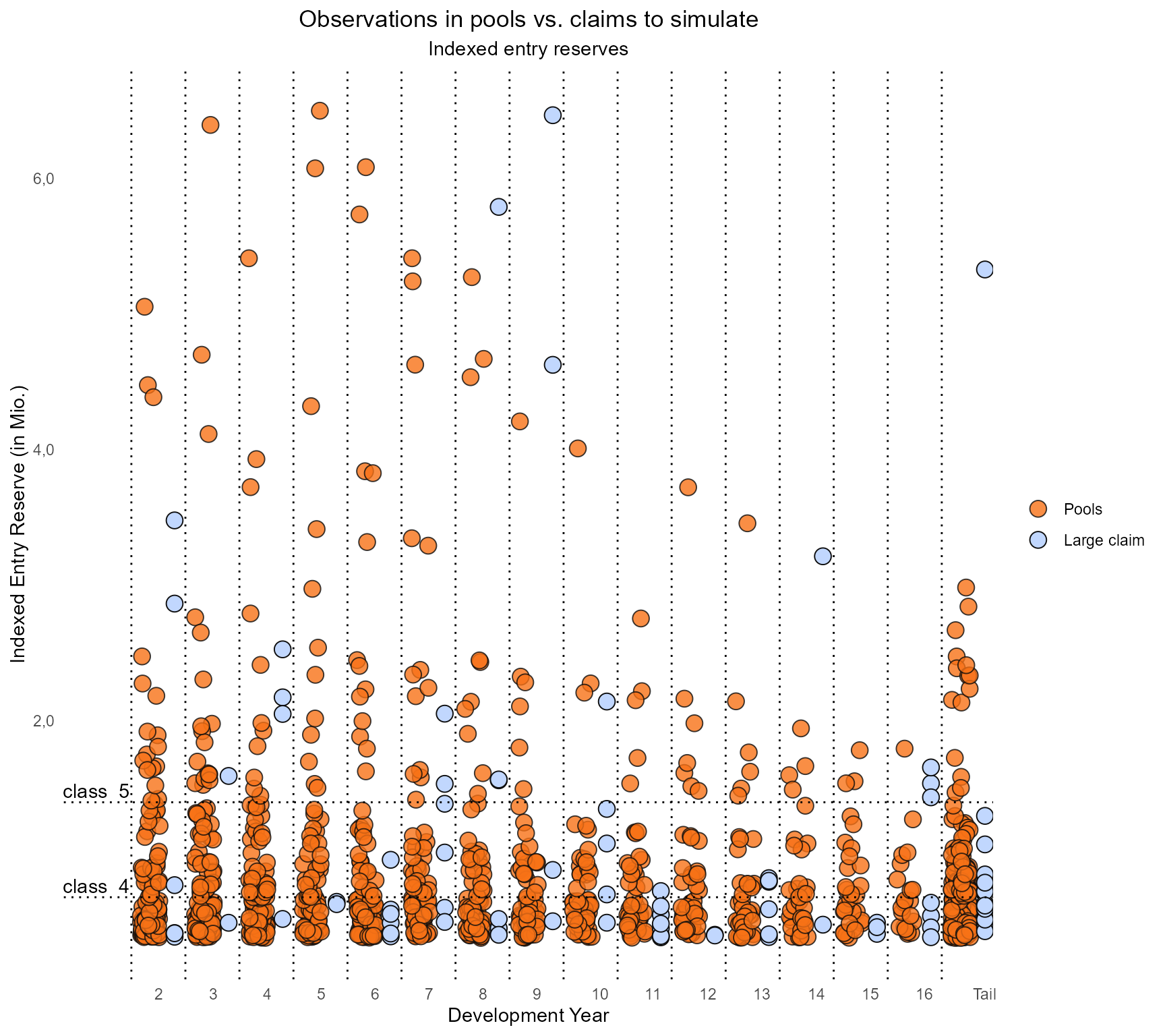
Note: The development year of the current large claims in the
plot is the first year to be simulated, so in the calendar year
last_orig_year it will be one year less.
The plot draws the historical observations of entry reserves on the left and the current large claims reserves on the right. This shows for which large claims there have only been very few similar claims in history. In this example, one claim in development year 8 of around 5.8 Mio. reserve, two in development year 9, one in development year 14 and one in the tail are obviously too big to be simulated with the observed history.
We extract the corresponding claim IDs from
extended_claims_data:
id1 <- extended_claims_data[extended_claims_data$Calendar_year == 2023 &
                               extended_claims_data$Dev_year_since_large == 7 &
                               extended_claims_data$Ind_cl_reserve > 5e6,]$Claim_id
id2 <- extended_claims_data[extended_claims_data$Calendar_year == 2023 &
                               extended_claims_data$Dev_year_since_large == 8 &
                               extended_claims_data$Ind_cl_reserve > 6e6,]$Claim_id
id3 <- extended_claims_data[extended_claims_data$Calendar_year == 2023 &
                               extended_claims_data$Dev_year_since_large == 8 &
                               extended_claims_data$Ind_cl_reserve > 4e6 &
                               extended_claims_data$Ind_cl_reserve < 6e6,]$Claim_id
id4 <- extended_claims_data[extended_claims_data$Calendar_year == 2023 &
                               extended_claims_data$Dev_year_since_large == 13 &
                               extended_claims_data$Ind_cl_reserve > 2e6,]$Claim_id
id5 <- extended_claims_data[extended_claims_data$Calendar_year == 2023 &
                               extended_claims_data$Dev_year_since_large > 15 &
                               extended_claims_data$Ind_cl_reserve > 4e6,]$Claim_id
special_claim_ids <- c(id1, id2, id3, id4, id5)
special_claim_ids
## [1] "Claim#3258" "Claim#3200" "Claim#3164" "Claim#2691" "Claim#1474"The plot can be updated with the special_claims dataframe, that is explained one chapter below:
plot_identify_special_claims(pools = pools,
                             extended_claims_data = extended_claims_data,
                             first_orig_year = first_orig_year,
                             last_orig_year = last_orig_year,
                             selected_reserve_classes = 3:5,
                             special_claims = data.frame(Claim_id = special_claim_ids,
                                                         Reserve2BE_percentage = 0.8,
                                                         Rollout_type = "linear"))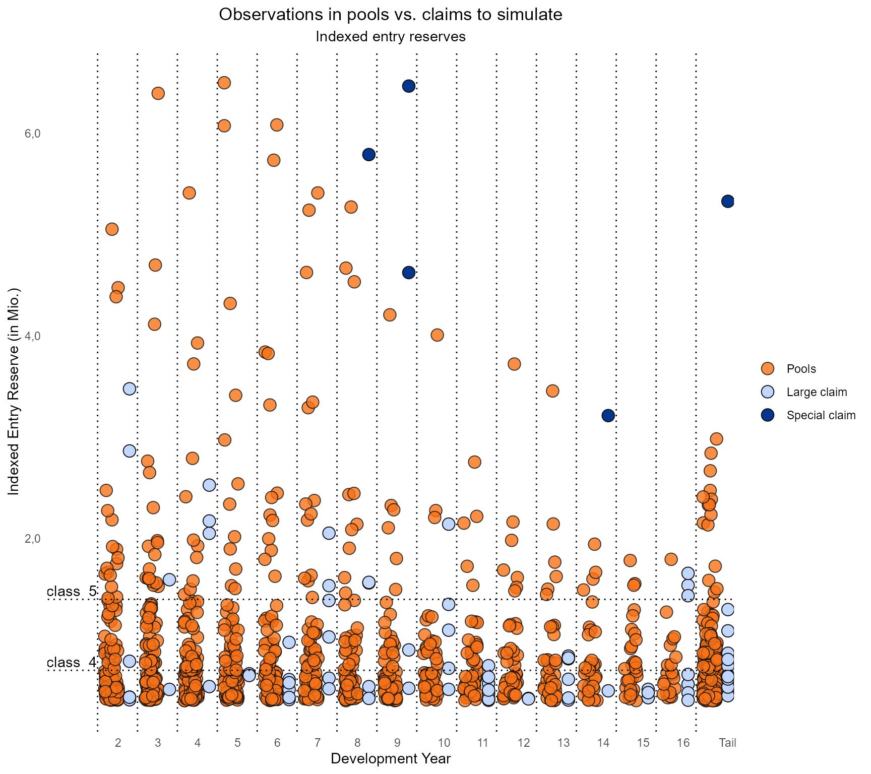
Others claims like in development year 2, 5, 7 or 10 are further candidates that need more detailed analysis. They will be treated as large claims here.
In the end, the decision about which claims to seperate from large claims to special claims has to be made by the responsible actuary and should in addition to the reserves include at least the claims’ development year and its overall development up to this point.
Dealing with special claims
Once the special claims are identified, they will be separated from the regular large claims and reserved deterministically:
- Active annuities are rolled out by multiplying the expected payments with the survival probabilities of the annuity recipient.
-
Claims reserves must be transitioned to a best
estimate and rolled out to the future. Thus, the dataframe
special_claimsneeds to be created with the following information:- Claim_id
- Reserve2BE_percentage with the information about how much of the reserve will be needed for the rest of the claim settlement.
-
Rollout_type with one of
linear,constantandexternal. In case ofexternalthe pattern_id must be defined in the column Pattern_id. - (Pattern_id An integer that refers to the entry of
the list
external_patternswhere concrete patterns may be chosen. As this is very rare for a specific claim in longtail business, we only use the rollout typelinearhere and set Reserve2BE_precentage to 80%.)
This is explained in more detail in the details section of
?compute_special_claims().
It is highly recommended to talk to the claims settlement department to estimate the future development of these claims.
special_claims <- data.frame(Claim_id = special_claim_ids,
                             Reserve2BE_percentage = 0.8,
                             Rollout_type = "linear")
special_claims
## Claim_id Reserve2BE_percentage Rollout_type
## 1 Claim#3258 0.8 linear
## 2 Claim#3200 0.8 linear
## 3 Claim#3164 0.8 linear
## 4 Claim#2691 0.8 linear
## 5 Claim#1474 0.8 linearNow the cashflows for the special claims can be computed.
special <- compute_special_claims(special_claims = special_claims,
                                  extended_claims_data = extended_claims_data,
                                  first_orig_year = first_orig_year,
                                  last_orig_year = last_orig_year,
                                  end_of_tail = 50,
                                  external_patterns = NULL,
                                  active_annuities = active_annuities_xmpl,
                                  age_shift = age_shift_xmpl,
                                  mortality = mortality_xmpl,
                                  reinsurance = reinsurance_xmpl,
                                  indices = indices_xmpl)
The resulting special is a list with matrices:
-
special_claims_paymentswith historic and future claim payments (250 + n columns) -
special_claims_reservedwith historic claims reserves (n columns) -
special_annuities_paymentswith historic and future annuity payments (250 + n columns) -
special_annuities_reservedwith historic annuities reserves (n columns) -
special_ceded_quota_paymentswith historic and future payments from the quota share reinsurance contract (250 + n columns) -
special_ceded_xl_paymentswith historic and future payments from the xl reinsurance contract (250 + n columns)
See ?compute_special_claims() for further information.
Here as an example the claim payments for the last two and the next 5
calendar years:
special$special_claims_payments[,c("2022", "2023", "2024", "2025", "2026", "2027", "2028")]## 2022 2023 2024 2025 2026 2027 2028
## 1989 0.00 0.00 0.0 0.0 0.0 0.0 0.0
## 1990 0.00 0.00 0.0 0.0 0.0 0.0 0.0
## 1991 0.00 0.00 0.0 0.0 0.0 0.0 0.0
## 1992 0.00 0.00 0.0 0.0 0.0 0.0 0.0
## 1993 0.00 0.00 0.0 0.0 0.0 0.0 0.0
## 1994 0.00 0.00 0.0 0.0 0.0 0.0 0.0
## 1995 0.00 0.00 0.0 0.0 0.0 0.0 0.0
## 1996 0.00 0.00 0.0 0.0 0.0 0.0 0.0
## 1997 0.00 0.00 0.0 0.0 0.0 0.0 0.0
## 1998 79125.31 60685.43 361239.0 346187.3 331135.7 316084.1 301032.5
## 1999 0.00 0.00 0.0 0.0 0.0 0.0 0.0
## 2000 0.00 0.00 0.0 0.0 0.0 0.0 0.0
## 2001 0.00 0.00 0.0 0.0 0.0 0.0 0.0
## 2002 0.00 0.00 0.0 0.0 0.0 0.0 0.0
## 2003 0.00 0.00 0.0 0.0 0.0 0.0 0.0
## 2004 0.00 0.00 0.0 0.0 0.0 0.0 0.0
## 2005 0.00 0.00 0.0 0.0 0.0 0.0 0.0
## 2006 0.00 0.00 0.0 0.0 0.0 0.0 0.0
## 2007 0.00 0.00 0.0 0.0 0.0 0.0 0.0
## 2008 0.00 0.00 0.0 0.0 0.0 0.0 0.0
## 2009 0.00 0.00 0.0 0.0 0.0 0.0 0.0
## 2010 0.00 0.00 0.0 0.0 0.0 0.0 0.0
## 2011 21145.58 56457.99 143344.4 139470.2 135596.1 131721.9 127847.7
## 2012 0.00 0.00 0.0 0.0 0.0 0.0 0.0
## 2013 0.00 0.00 0.0 0.0 0.0 0.0 0.0
## 2014 0.00 0.00 0.0 0.0 0.0 0.0 0.0
## 2015 272146.64 308892.21 182309.8 177969.1 173628.3 169287.6 164946.9
## 2016 486289.88 1210905.39 477873.8 466619.3 455364.9 444110.4 432856.0
## 2017 0.00 0.00 0.0 0.0 0.0 0.0 0.0
## 2018 0.00 0.00 0.0 0.0 0.0 0.0 0.0
## 2019 0.00 0.00 0.0 0.0 0.0 0.0 0.0
## 2020 0.00 0.00 0.0 0.0 0.0 0.0 0.0
## 2021 0.00 0.00 0.0 0.0 0.0 0.0 0.0
## 2022 0.00 0.00 0.0 0.0 0.0 0.0 0.0
## 2023 0.00 0.00 0.0 0.0 0.0 0.0 0.0Large claims
You find more information about the following functions in their help documentation.
Prepare simulation
To prepare the large claims simulation, we reduce
extended_claims_data to large claims:
large_extended_claims_data <-
   extended_claims_data[!extended_claims_data$Claim_id %in% special_claims$Claim_id,]
To simulate IBNR claims and reinsurance, the history needs to be created per single claim:
claims_history <- generate_history_per_claim(data = large_extended_claims_data,
                                             column = "Cl_payment_cal",
                                             first_orig_year = first_orig_year,
                                             last_orig_year = last_orig_year)
annuities_history <- generate_history_per_claim(data = large_extended_claims_data,
                                                column = "An_payment_cal",
                                                first_orig_year = first_orig_year,
                                                last_orig_year = last_orig_year)
history <- claims_history + annuities_history
history[1:10,1:5]
## Calendar_year
## Claim_id 1989 1990 1991 1992 1993
## Claim#535 25526.42384 3669.36920 553.05701 1831.06623 761.33266
## Claim#536 12230.61184 75.87735 17370.63663 26661.64539 11358.54477
## Claim#537 11182.00171 632.28564 4279.28325 24293.41598 8880.96316
## Claim#538 14036.18841 20560.77884 0.00000 0.00000 25124.25292
## Claim#539 941.79396 9051.06092 6959.30236 408.20552 187.42339
## Claim#540 759.04716 10949.55086 100794.55404 5797.28811 2784.66923
## Claim#541 66.37122 8874.99632 11478.68499 4420.23819 248571.13744
## Claim#548 12722.03674 41334.83196 14719.65272 2387.56055 22784.57107
## Claim#556 176.19904 46705.90023 54146.30042 7744.09055 37375.42832
## Claim#557 0.00000 11793.99346 41484.17418 15429.34294 0.00000The last required object is large_claims_list which is a
filtered and reduced version of
large_extended_claims_data.
large_claims_list <- generate_claims_list(extended_claims_data = large_extended_claims_data,
                                          first_orig_year = first_orig_year,
                                          last_orig_year = last_orig_year)
out(large_claims_list)
Simulation
After this preparation the simulation can be started:
sim_result <-  sicr(n = 10,
                    large_claims_list = large_claims_list,
                    first_orig_year = first_orig_year,
                    last_orig_year = last_orig_year,
                    pools = pools,
                    indices = indices_xmpl,
                    history = history,
                    exposure = exposure_xmpl,
                    years_for_ibnr_pools = 2014:2023,
                    active_annuities = active_annuities_xmpl,
                    age_shift = age_shift_xmpl,
                    mortality = mortality_xmpl,
                    reinsurance = reinsurance_xmpl,
                    progress = FALSE, # chose true to see progress during simulation
                    summary = TRUE)
##
##
## Gross Best Estimate: 115.855.799,30 (standard error: 1,57%)
## ...Known claims 96.166.746,02
## ...Claims 85.411.477,42
## ...Active annuities 7.567.455,99
## ...Future annuities 3.187.812,61
## ...IBNR 19.689.053,27
##
## Reinsurance Best Estimate: 41.180.612,37 (standard error (only XL): 6,70%)
## ...Known Claims 36.444.573,98
## ...XL 6.579.217,96
## ...Quota Share 29.865.356,02
## ...IBNR 4.736.038,39
## ...XL 252.293,75
## ...Quota Share 4.483.744,65The parameter years_for_ibnr_pools determines the
calendar years that shall be taken into account for IBNR claims.
sim_result is an array with one matrix for:
- Sum of gross payments
- Sum of reinsurance payments
- Claim payments (without annuity payments)
- Payments for active annuities
- Payments for expected future annuities
- Reinsurance payments from xl treaties
- Reinsurance payments from quota share treaties
Each matrix contains one row per known claim plus one row per expected IBNR claim and 250 columns for future calendar years.
As an example, this shows the overall gross payments for the next 5 years for the last 50 claims:
n <- nrow(sim_result)
sim_result[(n - 50):n, 1:5, "Gross_sum"]
## 2024 2025 2026 2027 2028
## Claim#3603 50537.03 22653.509 48695.530 82162.642 20492.206
## Claim#3611 39390.91 4552.862 16471.688 16569.343 3374.786
## Claim#3624 42405.89 32598.029 11888.435 12237.733 5458.804
## Claim#3631 55452.24 52412.193 8122.437 10211.108 -6594.378
## Claim#3643 27551.63 22045.364 52690.109 37169.988 9711.624
## Claim#3652 299503.90 167711.839 -161132.207 100162.724 79817.547
## Claim#3655 101614.23 108690.961 36581.927 22414.485 12578.747
## Claim#3662 223293.91 399616.456 -64310.454 70832.313 60921.835
## Claim#3674 53955.03 65491.046 18766.778 69518.794 66102.670
## IBNR1 105484.57 60300.668 35217.903 3921.545 18557.411
## IBNR2 93106.08 29046.155 32866.627 13827.160 15745.980
## IBNR3 96276.75 50442.898 61842.868 15335.102 33865.922
## IBNR4 105669.01 45356.880 42418.008 9448.106 18473.220
## IBNR5 73729.47 41463.099 50865.554 8826.979 12422.384
## IBNR6 0.00 90616.984 46764.104 76243.972 -96845.219
## IBNR7 0.00 0.000 58388.824 35367.519 55752.439
## IBNR8 0.00 0.000 0.000 56512.320 78710.153
## IBNR9 0.00 0.000 0.000 0.000 75941.458
## IBNR10 0.00 0.000 0.000 0.000 0.000
## IBNR11 0.00 0.000 0.000 0.000 0.000
## IBNR12 44334.54 28314.520 38387.669 15030.839 24626.126
## IBNR13 105872.63 65912.337 75355.569 25875.129 23662.181
## IBNR14 0.00 70839.551 26050.627 23508.048 29857.398
## IBNR15 0.00 0.000 0.000 147389.809 44418.217
## IBNR16 0.00 0.000 0.000 0.000 62702.886
## IBNR17 0.00 0.000 0.000 0.000 0.000
## IBNR18 0.00 0.000 0.000 0.000 0.000
## IBNR19 83980.30 17572.034 98717.826 34719.115 21923.123
## IBNR20 0.00 54563.827 34199.388 30833.257 10364.252
## IBNR21 0.00 0.000 0.000 56478.083 182422.885
## IBNR22 0.00 0.000 0.000 0.000 0.000
## IBNR23 0.00 0.000 0.000 0.000 0.000
## IBNR24 51852.37 42676.568 30468.018 15860.497 21265.651
## IBNR25 0.00 0.000 54833.090 177109.597 25047.776
## IBNR26 0.00 0.000 0.000 0.000 0.000
## IBNR27 0.00 0.000 0.000 0.000 0.000
## IBNR28 78402.04 40430.143 29988.803 23259.080 36034.590
## IBNR29 0.00 0.000 79516.442 79638.431 22709.520
## IBNR30 0.00 0.000 0.000 0.000 0.000
## IBNR31 0.00 60676.674 51905.885 35290.194 29010.266
## IBNR32 0.00 0.000 0.000 0.000 0.000
## IBNR33 0.00 52369.038 17650.025 7598.047 11448.534
## IBNR34 0.00 0.000 0.000 0.000 0.000
## IBNR35 0.00 0.000 0.000 28888.272 12156.365
## IBNR36 0.00 0.000 0.000 0.000 0.000
## IBNR37 0.00 0.000 0.000 0.000 0.000
## IBNR38 0.00 0.000 0.000 0.000 0.000
## IBNR39 0.00 0.000 0.000 0.000 0.000
## IBNR40 0.00 0.000 0.000 0.000 0.000
## IBNR41 0.00 0.000 0.000 0.000 0.000
## IBNR42 0.00 0.000 0.000 0.000 0.000At this stage, the single claim results can be used for a variety of analyses, for example for backtesting purposes. Some functions will be added soon to this package to create further plots with ggplot2 that support these tasks.
Aggregate single claims to origin years
We use the single claims results to aggregate to large claims results per origin year:
large <- aggregate_large_claims_results(
            sim_result = sim_result,
            large_claims_list = large_claims_list,
            large_extended_claims_data = large_extended_claims_data,
            history = history,
            reinsurance = reinsurance_xmpl,
            indices = indices_xmpl,
            first_orig_year = first_orig_year,
            last_orig_year = last_orig_year
)
The resulting large is a list with matrices:
-
large_claims_paymentswith historic and predicted claim payments (e.g. without annuities). -
large_claims_reservedwith historic claim reserves (without annuities). -
large_known_annuities_paymentswith historic and predicted payments for known annuities. -
large_annuities_reservedwith historic annuities’ reserves. -
large_future_annuities_paymentswith predicted payments for future annuities, the historic part is all 0. -
large_ibnr_paymentswith predicted payments for future annuities, the historic part is all 0. -
large_ceded_xl_paymentswith historic and predicted reinsurance payments for xl treaties. -
large_ceded_quota_paymentswith historic and predicted reinsurance payments for quota share treaties.
See ?aggregate_large_claims_results() for further
information. Here as an example the claim payments for the last two and
the next 3 calendar years:
large$large_claims_payments[, c("2022", "2023", "2024", "2025", "2026")]## 2022 2023 2024 2025 2026
## 1989 14277.658 11885.232 23582.81 32050.06 18849.081
## 1990 77686.419 52607.325 53420.68 27183.46 16120.461
## 1991 5796.983 6503.295 12314.09 25772.15 36753.991
## 1992 26725.487 17583.600 16390.78 16570.41 8715.902
## 1993 30265.710 17814.040 129197.73 63644.54 93349.968
## 1994 94721.250 154848.829 186941.39 163025.96 87995.168
## 1995 150430.001 84794.632 20217.07 51600.29 43854.425
## 1996 12864.412 10205.272 30902.44 26380.16 12800.903
## 1997 14183.457 -5254.346 47433.88 42584.80 15633.140
## 1998 36366.505 33754.697 71236.73 69175.12 73759.047
## 1999 38223.719 37029.380 69561.45 55828.26 61870.090
## 2000 23353.462 50644.146 78610.61 63459.00 167673.361
## 2001 39015.989 34303.684 74809.88 66777.52 51174.756
## 2002 27898.455 19120.069 32455.82 83816.86 65292.006
## 2003 99722.890 116610.325 98321.94 83154.66 62806.530
## 2004 202740.283 250054.750 24835.84 77323.05 109547.453
## 2005 21457.087 19815.160 163605.74 71920.23 65252.308
## 2006 74999.094 109415.226 138754.06 126407.72 108216.305
## 2007 194742.451 757793.802 349095.32 361972.73 91552.635
## 2008 30444.371 91372.511 105602.36 82386.57 112912.284
## 2009 309412.544 575420.758 321267.88 377759.52 386375.160
## 2010 196297.365 523662.661 118875.75 192268.07 98578.815
## 2011 77691.376 139535.563 142471.78 180659.46 122113.642
## 2012 222514.196 233028.729 268646.67 184057.61 116365.870
## 2013 271719.903 82217.747 75312.71 155292.32 82746.200
## 2014 305712.714 267582.346 399695.93 291642.61 376165.149
## 2015 490311.283 556094.325 433986.88 260226.64 355711.551
## 2016 780525.468 232128.978 251224.66 180429.06 210629.558
## 2017 556966.513 322315.694 472580.13 295779.74 191462.106
## 2018 931569.632 250583.016 714789.48 408025.52 417988.598
## 2019 441706.819 439999.492 230476.50 310986.69 315141.919
## 2020 759118.094 807989.786 607831.91 442848.10 435491.971
## 2021 1011918.824 1291582.348 336680.51 747080.32 563805.873
## 2022 102939.580 610207.211 244505.62 172595.20 159059.575
## 2023 0.000 89766.068 674355.94 737499.18 -174105.078Small claims
General description
Small claims can be derived as the difference between all claims and special + large claims.
The function compute_small_claims() computes all small
claim estimates in one step. This includes the following parts:
claim payments
Claim payments are projected via a standard chain ladder method. The possibility of reducing the used years for the chain ladder factors as well as the use of external patterns is implemented. As a standard, a paid method and an incurred method will be calculated and then aggregated as weighted sums.
The following parameters are required, all of them may be NULL which leads to the use of the standard chain paid and incurred chain ladder that are merged with equal weights.
- volume_paid_method: Number of newest calendar years to be used for paid chain ladder factors.
- volume_indurred_method: Number of newest calendar years to be used for incurred chain ladder factors.
-
external_paid_pattern: external pattern for paid
method, see
?generate_pattern()for usage. -
external_incurred_pattern: external pattern for
incurred method, see
?generate_pattern()for usage. -
int2ext_transition_paid: year of switching to
external paid pattern, see
?generate_pattern()for usage. -
int2ext_transition_incurred: year of switching to
external incurred pattern, see
?generate_pattern()for usage. -
weight_paid: weight of paid method for weighted
results, see
?merge_results()for usage. -
weight_incurred: weight of incurred method for
weighted results, see
?merge_results()for usage.
Calculation
small <- compute_small_claims(first_orig_year = first_orig_year,
                              last_orig_year = last_orig_year,
                              indices = indices_xmpl,
                              all_claims_paid = all_claims_paid_xmpl,
                              all_claims_reserved = all_claims_reserved_xmpl,
                              all_annuities_paid = all_annuities_paid_xmpl,
                              all_annuities_reserved = all_annuities_reserved_xmpl,
                              large_claims_list = large_claims_list,
                              large_claims_results = large,
                              special_claims = special_claims,
                              special_claims_results = special,
                              volume_paid_method = NULL,
                              volume_incurred_method = NULL,
                              external_paid_pattern = NULL,
                              external_incurred_pattern = NULL,
                              int2ext_transition_paid = NULL,
                              int2ext_transition_incurred = NULL,
                              weight_paid = 1,
                              weight_incurred = 1,
                              active_annuities = active_annuities_xmpl,
                              mortality = mortality_xmpl,
                              age_shift = age_shift_xmpl,
                              pool_of_annuities = pool_of_annuities_xmpl,
                              reinsurance = reinsurance_xmpl)
The resulting small is a list with matrices:
-
small_claims_paymentswith historic and predicted claim payments (e.g. without annuities). -
small_claims_reservedwith historic claim reserves (without annuities). -
small_known_annuities_paymentswith historic and predicted payments for known annuities. Historic payments are set to 0 ifall_annuities_paidisNULL. -
small_annuities_reservedwith historic annuities’ reserves. All entries are 0 ifsmall_annuities_reservedisNULL. -
small_future_annuities_paymentswith predicted payments for future annuities, the historic part is all 0. -
small_ceded_quota_paymentswith historic and predicted reinsurance payments for quota share treaties.
See ?compute_small_claims() for further information.
Here as an example the claim payments for the last two and the next 3
calendar years:
small$small_claims_payments[, c("2022", "2023", "2024", "2025", "2026")]## 2022 2023 2024 2025 2026
## 1989 0.0000 0.0000 675768.33 0.00 0.00
## 1990 3112.2328 4586.2047 261028.03 0.00 0.00
## 1991 389.8559 726.0541 341690.30 0.00 0.00
## 1992 1629.7160 1456.4997 387043.40 478287.95 0.00
## 1993 223.7702 22455.9312 106499.44 145113.84 179324.08
## 1994 11288.9299 0.0000 399324.43 31331.58 42691.74
## 1995 -328.6012 2524.7234 49706.71 311151.66 24413.42
## 1996 9429.8278 13282.1429 81265.66 53545.47 335181.33
## 1997 399.6041 3720.4524 72008.12 50123.23 33025.90
## 1998 9465.3362 12547.3199 30889.58 52846.36 36785.16
## 1999 -3660.9854 15005.4746 256743.23 47735.97 81667.41
## 2000 3010.2365 27525.9078 246717.60 237653.12 44186.57
## 2001 20314.5444 3169.0312 91120.63 102964.14 99181.21
## 2002 36632.9293 17942.0375 55060.85 105907.98 119673.50
## 2003 150755.5072 8224.6563 28896.59 28272.29 54380.94
## 2004 23569.3414 21137.5703 76644.48 47177.97 46158.70
## 2005 8460.7346 12889.2188 34351.19 20866.81 12844.42
## 2006 18733.1108 17063.5004 60522.61 76921.92 46726.61
## 2007 107837.1893 37372.1848 31666.32 30823.28 39175.20
## 2008 22197.8027 50594.3865 90081.41 57128.42 55607.51
## 2009 62661.4346 63226.3066 116517.58 119059.09 75505.67
## 2010 275276.8772 67741.5676 75178.31 74808.27 76440.01
## 2011 50350.1929 28492.5135 163723.67 81805.65 81402.99
## 2012 115221.6496 68434.2038 100612.09 105608.44 52767.98
## 2013 75432.0073 45737.3082 64597.18 62483.33 65586.22
## 2014 101156.9425 31703.2745 111660.60 70582.66 68272.93
## 2015 259150.0904 238541.1577 129736.02 106954.17 67607.64
## 2016 596861.2463 249966.8830 102441.16 69018.83 56899.01
## 2017 326726.6843 259953.4976 123542.26 91045.03 61340.79
## 2018 609755.5643 391256.1872 371758.28 250487.45 184597.87
## 2019 1106174.5642 667299.8601 421955.10 319284.33 215130.96
## 2020 1122738.8310 1018388.8060 590701.91 355572.71 269054.20
## 2021 5233697.4246 1859885.6245 708256.72 435012.14 261855.33
## 2022 10393654.0147 5430181.7121 1576165.21 914465.58 561665.88
## 2023 0.0000 9744646.6936 4620852.22 1350549.42 783566.95Substitute parts of the calculation
Every step may be replaced by alternative calculations, for example if chain ladder shall not be used or if another method for estimating future annuities appears more appropriate.
Read the code of compute_small_claims() for a step by
step guide in that case and replace the desired part.
Export to Excel
The package offers two functions to write the results into clearly
arranged excel worksheets. Both use openxlsx2:
- add_sicr_worksheet adds a worksheet to a workbook with payments and (optional) reserves as arguments
- add_sicr_aggr_worksheet adds an aggregated worksheet to a workbook from several existing worksheets, for example to add small, large and special claims to overall claims. Subtracting is also possible, for example to get the net view from gross and reinsurance payments.
The following example creates a complete results workbook with separating dummy worksheets and a reasonable order (small examples can be found in the functions documentation):
output <- openxlsx2::wb_workbook() %>%
   openxlsx2::wb_add_worksheet(sheet = "SMALL --->",
                               grid_lines = FALSE,
                               tab_color = openxlsx2::wb_color(hex = "#c85000")) %>%

   add_sicr_worksheet(sheetname = "SMALL claims",
                      payments = small$small_claims_payments,
                      reserved = small$small_claims_reserved) %>%

   add_sicr_worksheet(sheetname = "SMALL known annuities",
                      payments = small$small_known_annuities_payments,
                      reserved = small$small_annuities_reserved) %>%

   add_sicr_worksheet(sheetname = "SMALL future annuities",
                      payments = small$small_future_annuities_payments) %>%

   add_sicr_aggr_worksheet(sheetname = "SMALL gross",
                           sheets_to_add = c("SMALL claims",
                                             "SMALL known annuities",
                                             "SMALL future annuities")) %>%

   add_sicr_worksheet(sheetname = "SMALL ceded",
                      payments = small$small_ceded_quota_payments) %>%

   add_sicr_aggr_worksheet(sheetname = "SMALL net",
                           sheets_to_add = c("SMALL gross"),
                           sheets_to_subtract = c("SMALL ceded")) %>%

   openxlsx2::wb_add_worksheet(sheet = "LARGE --->",
                               grid_lines = FALSE,
                               tab_color = openxlsx2::wb_color(hex = "#c85000")) %>%

   add_sicr_worksheet(sheetname = "LARGE claims",
                      payments = large$large_claims_payments,
                      reserved = large$large_claims_reserved) %>%

   add_sicr_worksheet(sheetname = "LARGE known annuities",
                      payments = large$large_known_annuities_payments,
                      reserved = large$large_annuities_reserved) %>%

   add_sicr_worksheet(sheetname = "LARGE future annuities",
                      payments = large$large_future_annuities_payments) %>%

   add_sicr_worksheet(sheetname = "LARGE ibnr",
                      payments = large$large_ibnr_payments) %>%

   add_sicr_aggr_worksheet(sheetname = "LARGE gross",
                           sheets_to_add = c("LARGE claims",
                                             "LARGE known annuities",
                                             "LARGE future annuities",
                                             "LARGE ibnr")) %>%

   add_sicr_worksheet(sheetname = "LARGE ceded quota",
                      payments = large$large_ceded_quota_payments) %>%

   add_sicr_worksheet(sheetname = "LARGE ceded xl",
                      payments = large$large_ceded_xl_payments) %>%

   add_sicr_aggr_worksheet(sheetname = "LARGE ceded",
                           sheets_to_add = c("LARGE ceded quota",
                                             "LARGE ceded xl")) %>%

   add_sicr_aggr_worksheet(sheetname = "LARGE net",
                           sheets_to_add = c("LARGE gross"),
                           sheets_to_subtract = c("LARGE ceded")) %>%

   openxlsx2::wb_add_worksheet(sheet = "SPECIAL --->",
                               grid_lines = FALSE,
                               tab_color = openxlsx2::wb_color(hex = "#c85000")) %>%

   add_sicr_worksheet(sheetname = "SPECIAL claims",
                      payments = special$special_claims_payments,
                      reserved = special$special_claims_reserved) %>%

   add_sicr_worksheet(sheetname = "SPECIAL known annuities",
                      payments = special$special_annuities_payments,
                      reserved = special$special_annuities_reserved) %>%

   add_sicr_aggr_worksheet(sheetname = "SPECIAL gross",
                           sheets_to_add = c("SPECIAL claims",
                                             "SPECIAL known annuities")) %>%

   add_sicr_worksheet(sheetname = "SPECIAL ceded quota",
                      payments = special$special_ceded_quota_payments) %>%

   add_sicr_worksheet(sheetname = "SPECIAL ceded xl",
                      payments = special$special_ceded_xl_payments) %>%

   add_sicr_aggr_worksheet(sheetname = "SPECIAL ceded",
                           sheets_to_add = c("SPECIAL ceded quota",
                                             "SPECIAL ceded xl")) %>%

   add_sicr_aggr_worksheet(sheetname = "SPECIAL net",
                           sheets_to_add = c("SPECIAL gross"),
                           sheets_to_subtract = c("SPECIAL ceded")) %>%

   openxlsx2::wb_add_worksheet(sheet = "OVERALL --->",
                               grid_lines = FALSE,
                               tab_color = openxlsx2::wb_color(hex = "#c85000")) %>%

   add_sicr_aggr_worksheet(sheetname = "OVERALL gross",
                           sheets_to_add = c("SMALL gross",
                                             "LARGE gross",
                                             "SPECIAL gross")) %>%

   add_sicr_aggr_worksheet(sheetname = "OVERALL ceded",
                           sheets_to_add = c("SMALL ceded",
                                             "LARGE ceded",
                                             "SPECIAL ceded")) %>%

   add_sicr_aggr_worksheet(sheetname = "OVERALL net",
                           sheets_to_add = c("OVERALL gross"),
                           sheets_to_subtract = c("OVERALL ceded")) %>%

   openxlsx2::wb_add_worksheet(sheet = "LIFE NONLIFE --->",
                               grid_lines = FALSE,
                               tab_color = openxlsx2::wb_color(hex = "#c85000")) %>%

   add_sicr_aggr_worksheet(sheetname = "LIFE gross",
                           sheets_to_add = c("SMALL known annuities",
                                             "SMALL future annuities",
                                             "LARGE known annuities",
                                             "LARGE future annuities",
                                             "SPECIAL known annuities")) %>%

   add_sicr_aggr_worksheet(sheetname = "NONLIFE gross",
                           sheets_to_add = c("OVERALL gross"),
                           sheets_to_subtract = c("LIFE gross")) %>%

   openxlsx2::wb_set_order(
         c("OVERALL --->", "OVERALL gross", "OVERALL ceded", "OVERALL net",
           "LIFE NONLIFE --->", "LIFE gross", "NONLIFE gross",
           "SMALL --->", "SMALL claims", "SMALL known annuities", "SMALL future annuities",
               "SMALL gross", "SMALL ceded", "SMALL net",
           "LARGE --->", "LARGE claims", "LARGE known annuities", "LARGE future annuities", "LARGE IBNR",
               "LARGE gross", "LARGE ceded quota", "LARGE ceded xl", "LARGE ceded", "LARGE net",
           "SPECIAL --->", "SPECIAL claims", "SPECIAL known annuities",
               "SPECIAL gross", "SPECIAL ceded quota", "SPECIAL ceded xl", "SPECIAL ceded", "SPECIAL net"))
Save the output with
openxlsx2::wb_save(wb = output,
                   file = "output.xlsx")
or open it with
openxlsx2::wb_open(output)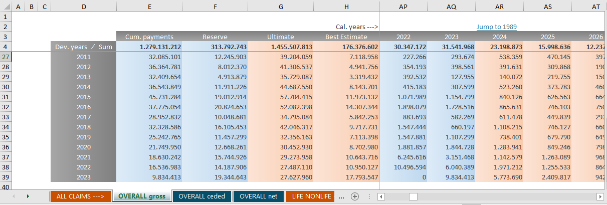
Useful plots
This package comes with some further plotting functions that have been useful in the past.
General information
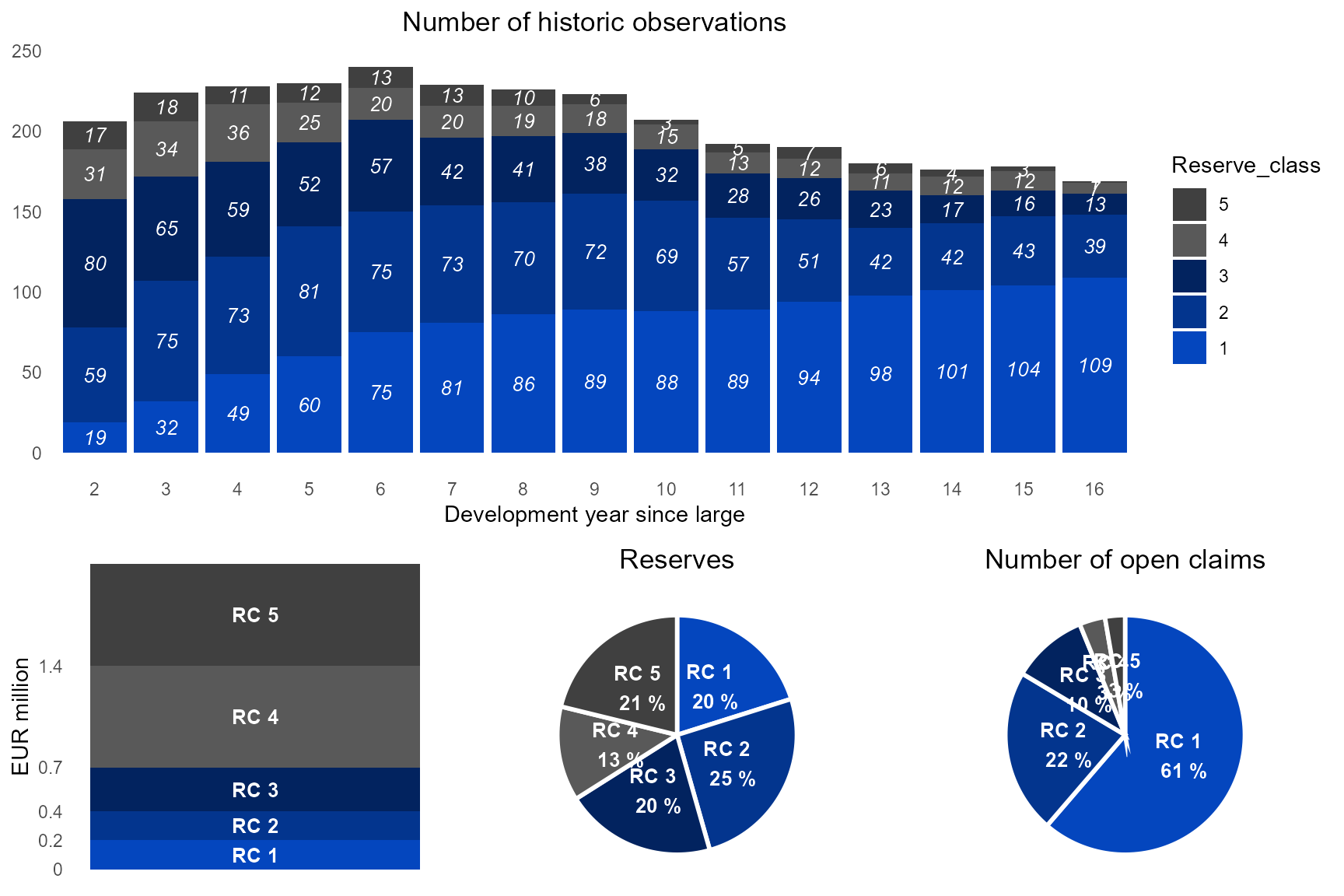
The first function returns four simple plots that describe the pools and reserve classes.
p_pools <- plot_pools_overview(pools, large_claims_list)
if (requireNamespace("gridExtra", quietly = TRUE)) {
   plot1 <- gridExtra::grid.arrange(p_pools[[1]],
                       gridExtra::arrangeGrob(p_pools[[2]], p_pools[[3]], p_pools[[4]], ncol = 3, widths = c(1,1,1)),
                       ncol = 1, heights = c(3, 2))
   plot1} else {
      print("gridExtra not installed. Only the first plot is shown.")
      p_pools[1]
   }
## TableGrob (2 x 1) "arrange": 2 grobs
##   z     cells    name            grob
## 1 1 (1-1,1-1) arrange  gtable[layout]
## 2 2 (2-2,1-1) arrange gtable[arrange]
Reserve vs Best Estimate comparison
After simulating you might want to see the difference between the original claim reserve and the predicted best estimate. The following functions creates two plots for this purpose, one per reserve class and one per development year.
p_reserve_vs_be <-
   plot_reserve_vs_be(large_claims_list = large_claims_list,
                      sim_result = sim_result)
p_reserve_vs_be[[1]]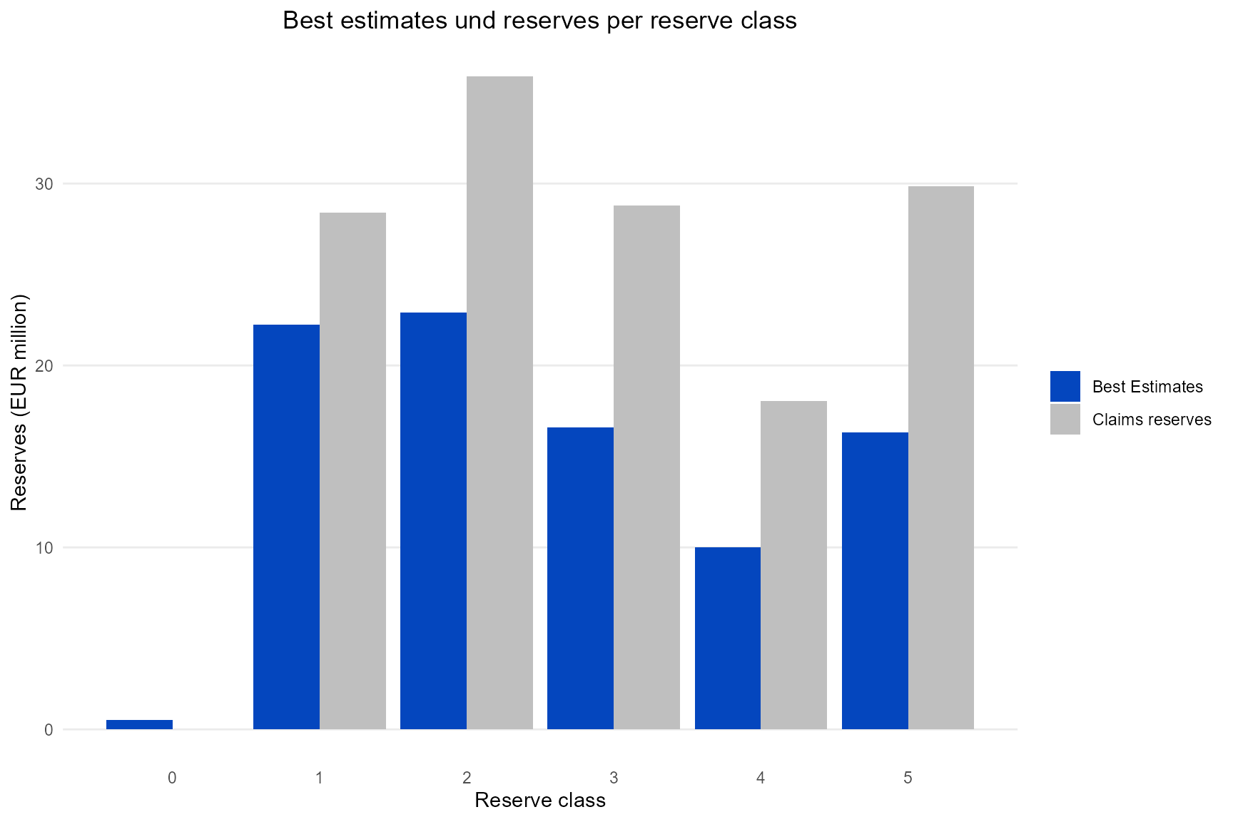
p_reserve_vs_be[[2]]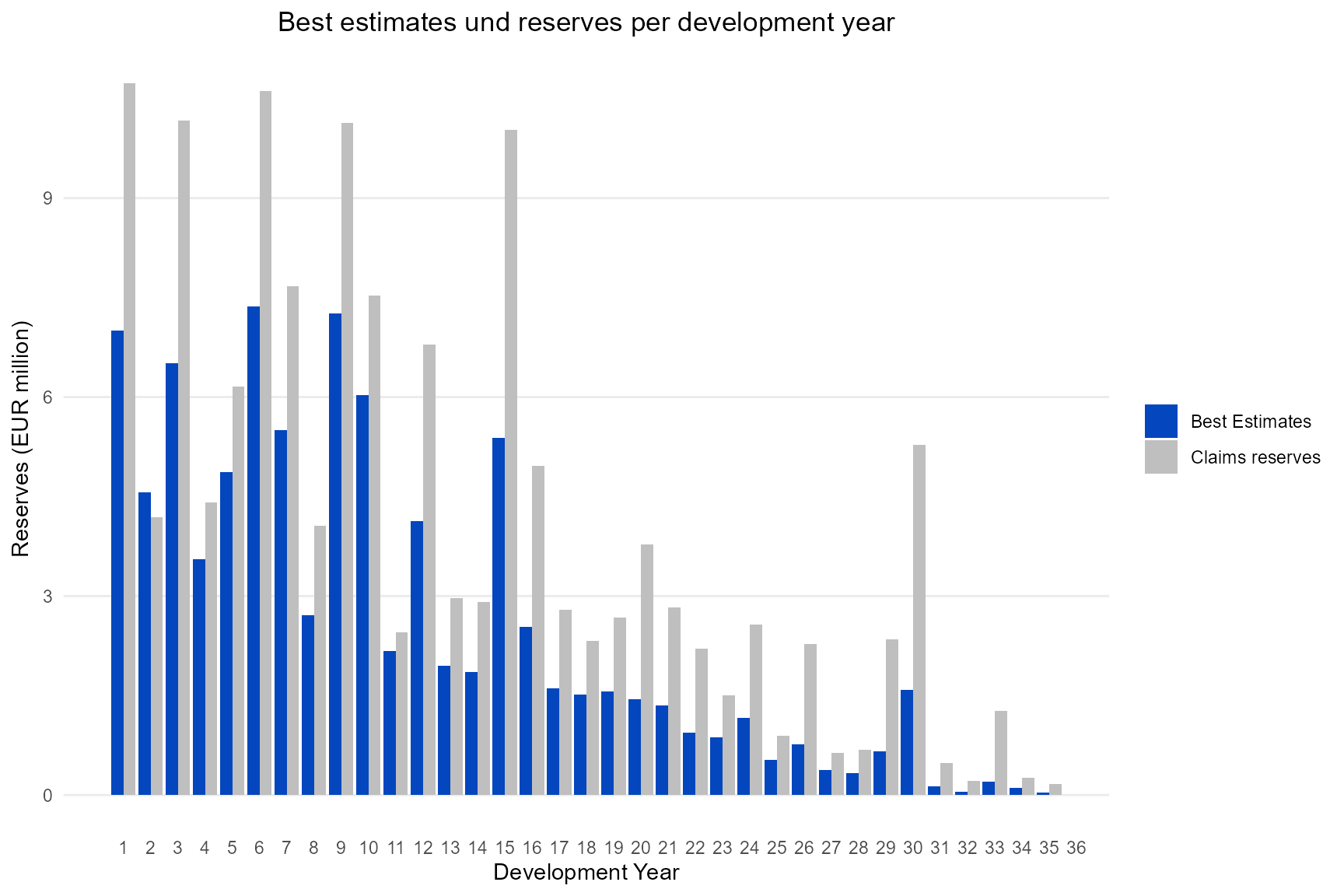
The following plots show this difference on a single claim basis. The first plot contains the pretail years, the second the tail years. The plot shows how the best estimates decrease with increasing development year. Note that the best estimates of the highest reserve class are not stable due to a reduced and fictive input claims dataset.
p_reserve_vs_be_single <-
   plot_reserve_vs_be_per_claim(last_orig_year = 2023,
                                pools = pools,
                                large_claims_list = large_claims_list,
                                indices = indices_xmpl,
                                age_shift = age_shift_xmpl,
                                mortality = mortality_xmpl)
p_reserve_vs_be_single[[1]]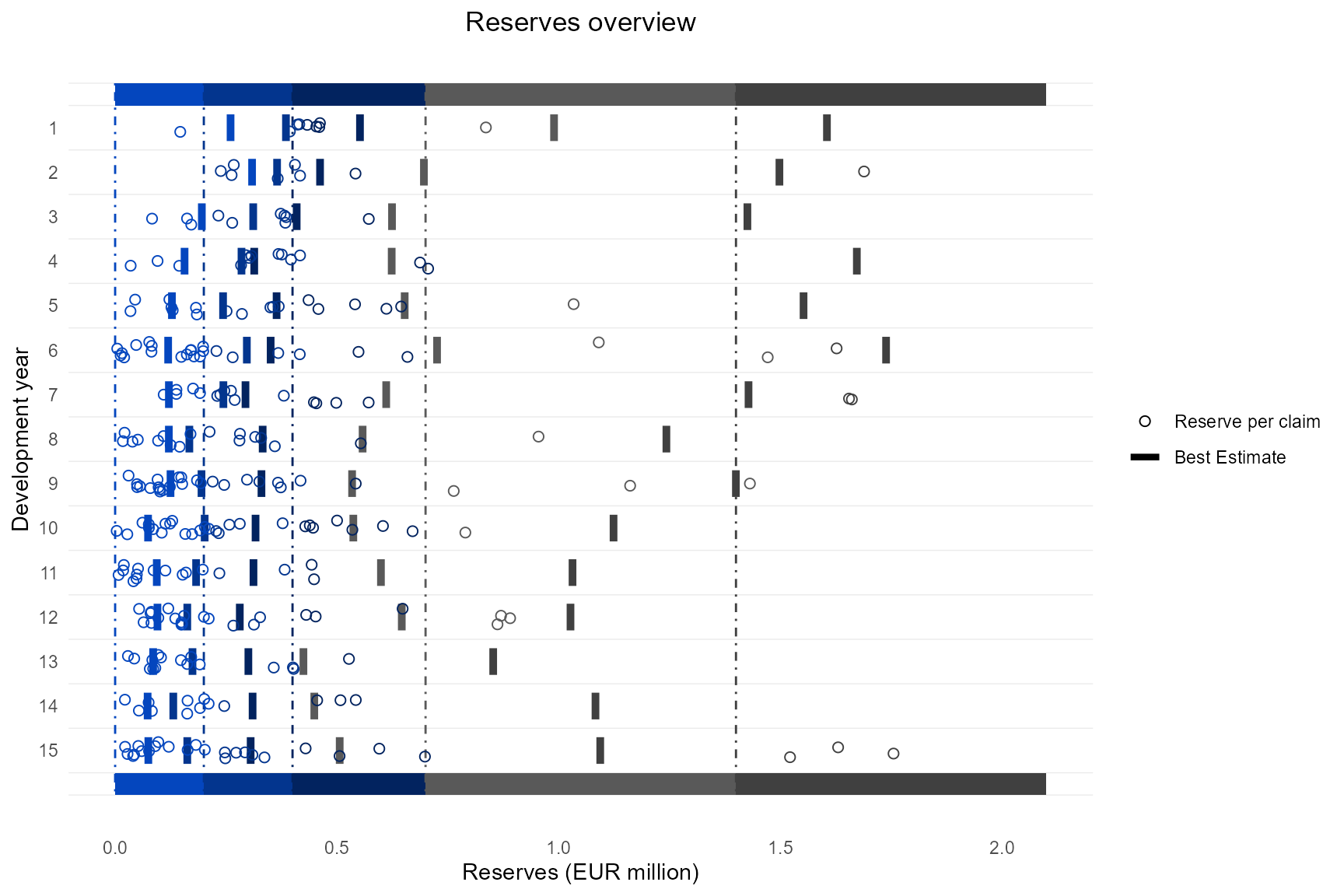
p_reserve_vs_be_single[[2]]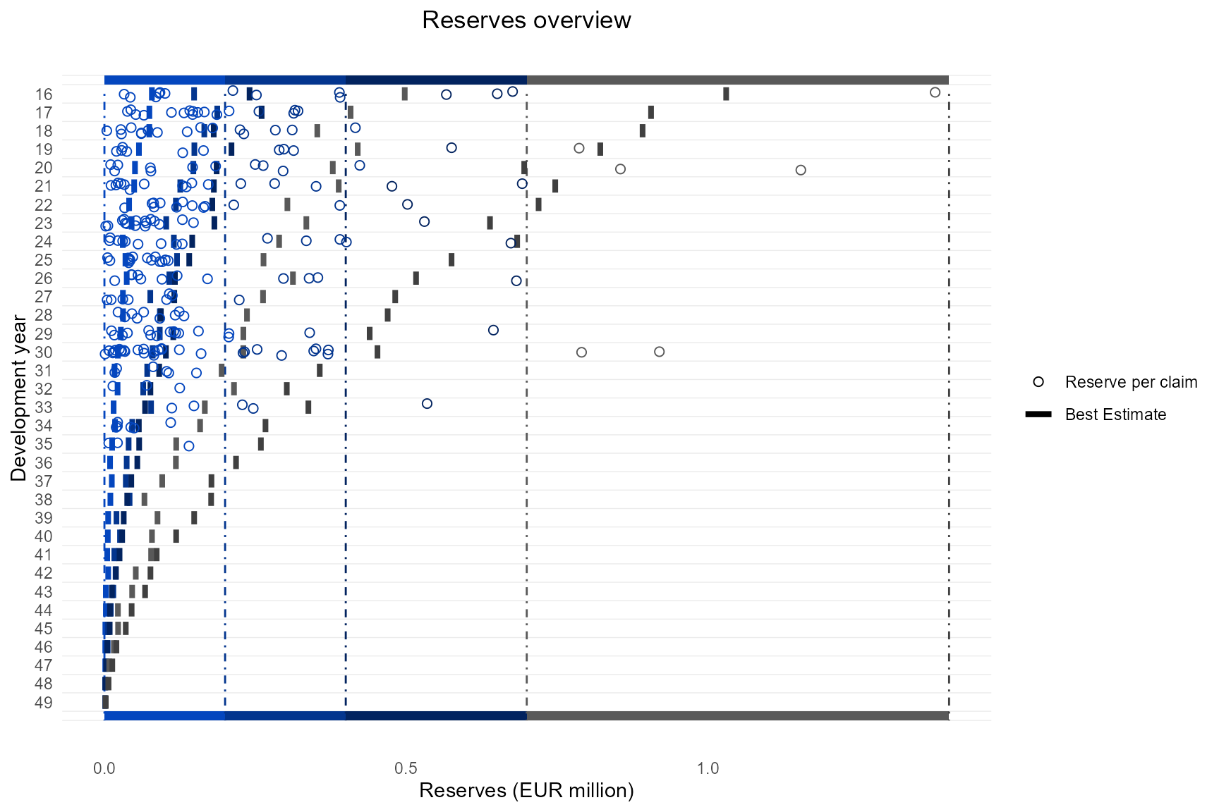
Backtesting
All the backtesting functions compare the actual payments with payments’ expectations and their quantiles. For this purpose we need to create a predicted payments series from the old reservation in advance.
Backtesting after one year
The most common backtesting compares the actual payments with the predicted payments from one year ago. The last origin year in this example is 2023. Therefore we need the predicted payments series from 2022 here.
claims_data_old <- dplyr::filter(claims_data_xmpl,
                                 Calendar_year <= 2022)

historic_indices_old <- dplyr::filter(historic_indices_xmpl,
                                      Calendar_year <= 2022)

indices_old <- expand_historic_indices(historic_indices_old,
                                       first_orig_year = 1989,
                                       last_orig_year = 2022,
                                       index_gross_future = 0.03,
                                       index_re_future = 0.02)

indices_old <- add_transition_factor(indices_old, index_year = 2022)
extended_claims_data <- prepare_data(claims_data = claims_data_old,
                                     indices = indices_old,
                                     threshold = 400000,
                                     first_orig_year = 1989,
                                     last_orig_year = 2022,
                                     expected_year_of_growing_large = 3,
                                     reserve_classes = c(1, 200001, 400001, 700001, 1400001),
                                     pool_of_annuities = pool_of_annuities_xmpl)

pools <- generate_pools(extended_claims_data = extended_claims_data,
                        reserve_classes = c(1, 200001, 400001, 700001, 1400001),
                        years_for_pools = 2014:2022,
                        start_of_tail = 17,
                        end_of_tail = 50,
                        lower_outlier_limit = -Inf,
                        upper_outlier_limit = Inf,
                        pool_of_annuities = pool_of_annuities_xmpl)

large_claims_list <- generate_claims_list(extended_claims_data = extended_claims_data,
                                          first_orig_year = 1989,
                                          last_orig_year = 2022)

history <- generate_history_per_claim(data = extended_claims_data,
                                      column = "Cl_payment_cal",
                                      first_orig_year = 1989,
                                      last_orig_year = 2022)

series <- sicr_series(n = 50,
                      large_claims_list = large_claims_list,
                      first_orig_year = 1989,
                      last_orig_year = 2022,
                      pools = pools,
                      indices = indices_old,
                      history = history,
                      progress = FALSE)
Now we derive the new extended_claims_data dataframe and create the plot:
extended_claims_data_new <- prepare_data(claims_data = claims_data_xmpl,
                                     indices = indices_xmpl,
                                     threshold = 400000,
                                     first_orig_year = 1989,
                                     last_orig_year = 2023,
                                     expected_year_of_growing_large = 3,
                                     reserve_classes = c(1, 200001, 400001, 700001, 1400001),
                                     pool_of_annuities = pool_of_annuities_xmpl)

g_oy <- backtesting_1y_per_origin_year(sim_result_series_old = series,
                                       extended_claims_data_new = extended_claims_data_new)
g_rc <- backtesting_1y_per_reserve_class(sim_result_series_old = series,
                                         extended_claims_data_new = extended_claims_data_new)
First per origin year:
g_oy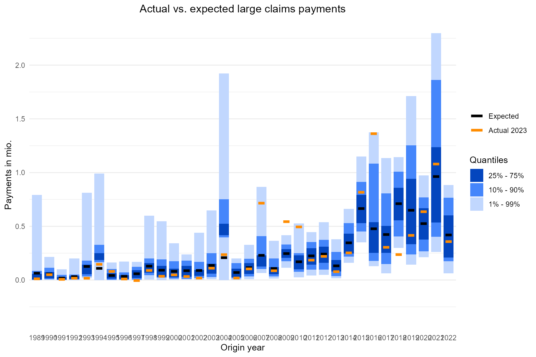
Then per reserve class:
g_rc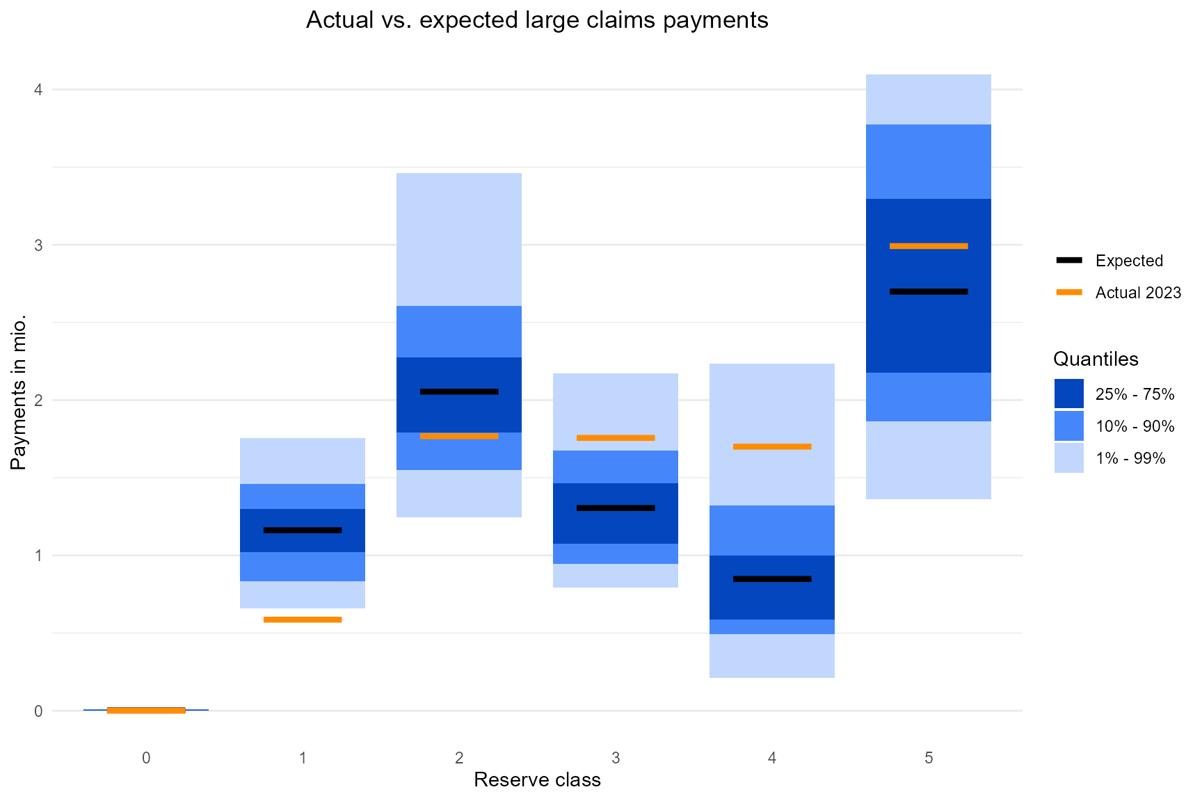
Another function offers a further zoom in to the payments’ expectation and quantiles for single claims. Chose a reserve class and the desired development years in the functions arguments. The points may either be labelled by the claim id or with the origin year. It will not be labelled at all if the ggrepel package is not installed.
In the following example we create the plot for reserve class 5 and development years 2:10.
g_single <- backtesting_1y_single_per_dev_year(sim_result_series_old = series,
                                               extended_claims_data_new = extended_claims_data_new,
                                               reserve_class = 4,
                                               dev_year = 2:10)
g_single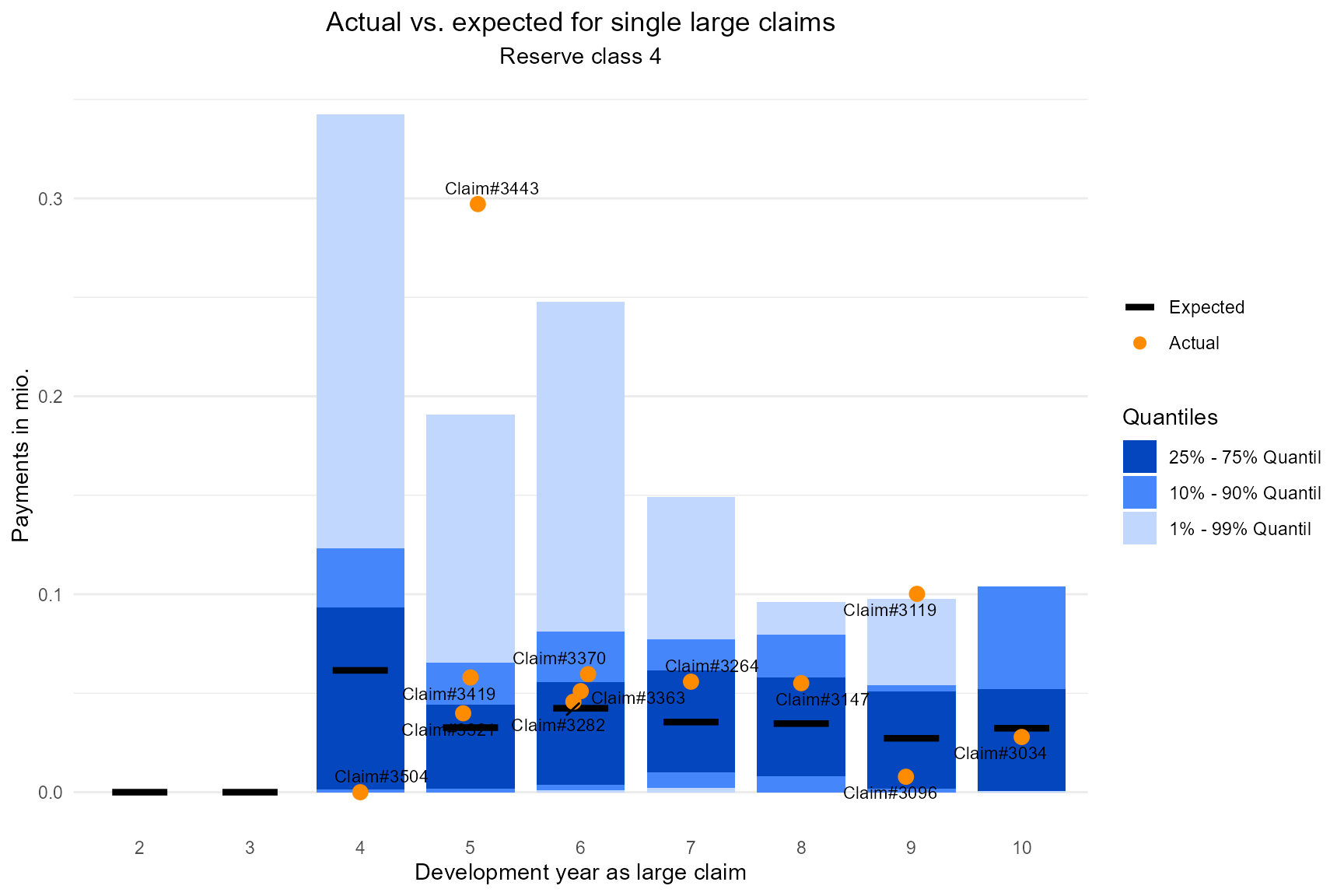
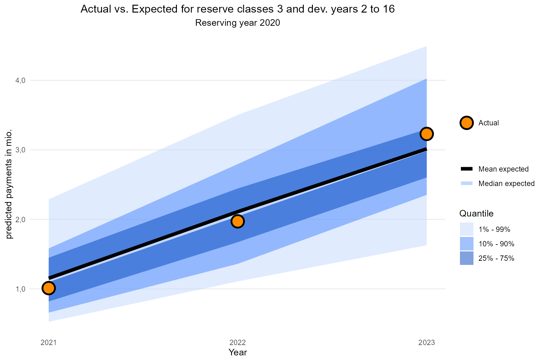
Multiyear backtesting
You might also be interested in an actual vs expected comparison over multiple years. For this purpose we create the above objects for an earlier reserving year (e.g. 2020) and build the plot:
claims_data_old <- dplyr::filter(claims_data_xmpl,
                                 Calendar_year <= 2020)

historic_indices_old <- dplyr::filter(historic_indices_xmpl,
                                      Calendar_year <= 2020)

indices_old <- expand_historic_indices(historic_indices_old,
                                       first_orig_year = 1989,
                                       last_orig_year = 2020,
                                       index_gross_future = 0.03,
                                       index_re_future = 0.02)

indices_old <- add_transition_factor(indices_old, index_year = 2022)
extended_claims_data <- prepare_data(claims_data = claims_data_old,
                                     indices = indices_old,
                                     threshold = 400000,
                                     first_orig_year = 1989,
                                     last_orig_year = 2020,
                                     expected_year_of_growing_large = 3,
                                     reserve_classes = c(1, 200001, 400001, 700001, 1400001),
                                     pool_of_annuities = pool_of_annuities_xmpl)
pools <- generate_pools(extended_claims_data = extended_claims_data,
                        reserve_classes = c(1, 200001, 400001, 700001, 1400001),
                        years_for_pools = 2014:2020,
                        start_of_tail = 17,
                        end_of_tail = 50,
                        lower_outlier_limit = -Inf,
                        upper_outlier_limit = Inf,
                        pool_of_annuities = pool_of_annuities_xmpl)

large_claims_list <- generate_claims_list(extended_claims_data = extended_claims_data,
                                          first_orig_year = 1989,
                                          last_orig_year = 2020)

history <- generate_history_per_claim(data = extended_claims_data,
                                      column = "Cl_payment_cal",
                                      first_orig_year = 1989,
                                      last_orig_year = 2020)

series <- sicr_series(n = 50,
                      large_claims_list = large_claims_list,
                      first_orig_year = 1989,
                      last_orig_year = 2020,
                      pools = pools,
                      indices = indices_old,
                      history = history,
                      progress = FALSE)

g_multiyears <- backtesting_multiyears(sim_result_series_old = series,
                                       extended_claims_data_new = extended_claims_data_new,
                                       reserve_classes = 3,
                                       dev_year = 2:16)
g_multiyears